Thursday, November 19, 2015

TACTIC Custom Tools and Plugins


INTRODUCTION

Our company builds web based casino games such as slot machines, video conferencing poker, roulettes, and all sorts of casino games. We build these games from inception, design, 2d/3d art assets, programming, to the final web site. There is already an existing base of games that needs to have its interface updated, as well as adding new games with new gameplay and eye candy that can attract players. The size of the projects also varies in size, there’s going to be one flagship game every year and a bunch of mid tier games and lots of smaller games. Besides the games itself, our department also need to provide commercials for these games in the form of computer animations. So there is a large variety of projects to consider. Our company have two 3d teams in house, one using 3dsmax and the other with Maya. 3dsmax users are primarily focused on game assets. While maya users could be tasked with games, animations, commericials.


PROJECT STRUCTURE

I started with Tactic version 4.1.3 and decided not to use the templates. The first thing I did is determing the project structure. By default Tactic seems to want the administrators to set each project as the top level. I decided against that and simply set our department(or just an abstract) as the top level. The main objectes to track are the projects, and with each project, depending on type, assets and/or shots. Projects will have pipelines consisting of marketing, concept, 3d, package, and RD, that tracks the project as it moves from department to department. Assets and Shots are a sub type of concept and 3d deprtment and will have pipelines that track assets through 2d/3d processes. 


FILE MANAGEMENT IN MAYA/MAX/NUKE INTEGRATION


Main UI
I did not particularly like the check-in check-out implemented in TACTIC. I spent too much time trying to get it to work or have any actual use. JAVA was being phased out of Chrome during 2014, and the check-in tool saw action for a couple of months, but had too many problems regarding unicode, UNC path and what not. In the end, check-ins were only used for images/videos, and the JAVA checkin tool is abandoned, and we only used HTML5 image/video check-in or check-ins using the Python API.So, instead of file management using check-ins, I developed a system that can check TACTIC for projects, its associated assets and shots, and its pipelines from Maya/Max/Nuke. The system provides folder naming convention and file naming convention based on TACTIC, and versioning based on files in the folder. As it is built with python and QT, I could run this tool from Maya/Max/Nuke. So once the project and its assets are determined and properly inputed into TACTIC, I can open up any DCC tool and the script, where I can find the project > object > process and either do the initial save, or open an existing file. Each time I save with the tool it increments the version. So there is no over writing with the tool. A little bit of info is also retrieved and displayed in the tool for convenience sake as well. 
These buttons filters projects that are currently in progress, ready, or completed projects. 

This button says ‘Update Cache’. Since I need three lists of projects(in progress, ready, complete), I need to query and search TACTIC three times, but that takes too long. So what I did was to write out three separate lists to a table on tactic, and read from their instead. So instead of a search, it simply retrieves the lists. This cache is updated daily, but can also be updated manually with this button. 

Here is the main interface, choosing projects will show which items are available to work on. The user can choose assets or shots. Choosing items will show pipeline processes, in this case, model and rigging. 

These are supplementatry information, the left pane displays project name, project type, project coordinator, start date, end date. The right pane displays item name, item type, assigned, start date, end date.
The first row is the login name, corresponding button logs out the user and shows a login menu. 
The second row displays the generated folder path, the rule here is {project name}/{assets/shots}/{item_type}/{item_name}/{process}/ and then a unified maya/max/nuke folder structure, where its basically an input folder for textures, or plates for nuke, an output folder for renders, a scenes folder for the work files, and a data folder for cache, misc data, hair, garbage, etc. The corresponding button opens the path in file explorer. 
The last row displays the generated filename, the rule here is, {abbreviation of project name}_{abbreviation of item_type}_{item_name}_{abbreviation of process}_{version}_{author}.{mb, max, or nk}. The corresponding button saves the file. The script knows the application that opened it, so it will load the corresponding API(maya.cmds, Maxplus, or Nuke), and use the appropriate command. It will also set the project environment for each application.
This is the files pane, picking any file and press open, opens the file. Publish could either check the file into TACTIC, or copy the file up a level as a master file. Function not yet determined, and not really essential.
From here on out, a lot of automation can be introduced, for example quick renders directly to TACTIC, render farm outputs to TACTIC. Which brings us, to my next tool.

DAILIES TOOL V01

Instead of checking in files to TACTIC for version control, we adapted the checkin for Quality control/dailies. This tool is a custom layout in TACTIC that first displays a tile view of current projects, which can be quickly sorted and filtered, and then displays the assets and shots of the selected project. The display is two dimensional, where left and right cycles through the items, while up and down cycles through all the images/videos of that particular items through out its pipeline. This tool combines custom layout, python, javascript, jquery, and reveal.js. 


The structure of this one is quite interesting, it is a custom layout that loads a list of project using python through mako. The python script builds the main page by appending HTML to a massive string. Using the Javascript Behaviors in custom layout, it takes project information and filter settings from the page and runs server.execute_command() to execute another python script that builds the reveal.js interface. This python script generates a HTML string and returns it to JS which is prepended into the top of the DOM. 


Figure 1 Dailies Selection Page

The top left tool bar are filters to filter out projects based on project type and item type. Choosing item type will show only items of that type in the dailies page.  


Figure 2

 Title PageClicking on a project will enter the dailies page. Here is the title page. 


Figure 3 Overview

By pressing ESC we enter overview of the dailies page. Since its hard to demonstrate the structure in each slide, we’ll look at the over all structure of the dailies tool. As we can see, items are listed horizontally, while history of each item is listed vertically. History is sorted by time, and then by pipeline process. So the newest image or video of the latest process will always be on top. Navigation are using arrow keys or the joy pad at the right bottom of the screen.  


Figure 4 Image View

This is the actual dailies view based on reveal js. One of the challenges is gettings CSS to work with reveal js AND TACTIC. Formatting CSS under a TACTIC table is quite a challenge. In the end, I just prepend everything to the top of the DOM and attach a separate CSS file while in the dailies view. Loading images and videos takes at least 2 to 3 seconds, as it needs to search through project type > project items > snapshots > files. 

So this is our automated quality control and dailies tool I have implemented. Currently in development is a better lightbox and UI design where I can zoom in/out and pan the images. The standalone tool is built already but I haven’t had time to integrate it into TACTIC yet. 

RENDERFARM UTILIZATION TO TACTIC


Our renderfarm, also setup by me, are blades running ESXI hypervisors managed with VSphere. Although blade and cluster utilization information are readily availabe in VSphere, management required a more user friendly interface then logging into VSphere Center and finding the settings to display utilization data. Since it is only a tool to assess farm capacity, it does not require real time data. Instead, I used PyVmomi to write out Vsphere data to TACTIC daily. From there, I used Highcharts.js to render out Cluster Utilization. The top chart are 16 blades divided into 4 clustes allocated to 4 departments. So each department has access to at least one cluster. The bottom chart are retired workstations serving as additional capacity.


Highcharts is pretty cool in that I can zoom in to a particular range in time.  


MODEL, ANIMATION DATABASE


I have also built an model and animation database into our TACTIC Server. Models and animations are acquired from both free and paid websites.  Using Selenium to scrape files, thumbnails, and information. All of these is then compiled into TACTIC where it can be keyword searched, or browsed by category. The top left bar filters out the models based on model type, and each model type has sub types as well. For example, the image below has Furniture Selected, with sub types of chairs, tables, beds, etc etc. 

There are currently 44044 models in the model database and 2236 animations in the animation database. Clicking on the tile downloads the zip or fbx file. This behavior is modified in tile_layout_wdg.py. 


Monday, November 16, 2015

Postgres Comands

General

\copyright show PostgreSQL usage and distribution terms
\g [FILE] or ; execute query (and send results to file or |pipe)
\gset [PREFIX] execute query and store results in psql variables
\h [NAME] help on syntax of SQL commands, * for all commands
\q quit psql
\watch [SEC] execute query every SEC seconds

Query Buffer

\e [FILE] [LINE] edit the query buffer (or file) with external editor
\ef [FUNCNAME [LINE]] edit function definition with external editor
\p show the contents of the query buffer
\r reset (clear) the query buffer
\s [FILE] display history or save it to file
\w FILE write query buffer to file

Input/Output

\copy ... perform SQL COPY with data stream to the client host
\echo [STRING] write string to standard output
\i FILE execute commands from file
\ir FILE as \i, but relative to location of current script
\o [FILE] send all query results to file or |pipe
\qecho [STRING] write string to query output stream (see \o)

Informational

(options: S = show system objects, + = additional detail)
\d[S+] list tables, views, and sequences
\d[S+] NAME describe table, view, sequence, or index
\da[S] [PATTERN] list aggregates
\db[+] [PATTERN] list tablespaces
\dc[S+] [PATTERN] list conversions
\dC[+] [PATTERN] list casts
\dd[S] [PATTERN] show object descriptions not displayed elsewhere
\ddp [PATTERN] list default privileges
\dD[S+] [PATTERN] list domains
\det[+] [PATTERN] list foreign tables
\des[+] [PATTERN] list foreign servers
\deu[+] [PATTERN] list user mappings
\dew[+] [PATTERN] list foreign-data wrappers
\df[antw][S+] [PATRN] list [only agg/normal/trigger/window] functions
\dF[+] [PATTERN] list text search configurations
\dFd[+] [PATTERN] list text search dictionaries
\dFp[+] [PATTERN] list text search parsers
\dFt[+] [PATTERN] list text search templates
\dg[+] [PATTERN] list roles
\di[S+] [PATTERN] list indexes
\dl list large objects, same as \lo_list
\dL[S+] [PATTERN] list procedural languages
\dm[S+] [PATTERN] list materialized views
\dn[S+] [PATTERN] list schemas
\do[S] [PATTERN] list operators
\dO[S+] [PATTERN] list collations
\dp [PATTERN] list table, view, and sequence access privileges
\drds [PATRN1 [PATRN2]] list per-database role settings
\ds[S+] [PATTERN] list sequences
\dt[S+] [PATTERN] list tables
\dT[S+] [PATTERN] list data types
\du[+] [PATTERN] list roles
\dv[S+] [PATTERN] list views
\dE[S+] [PATTERN] list foreign tables
\dx[+] [PATTERN] list extensions
\dy [PATTERN] list event triggers
\l[+] [PATTERN] list databases
\sf[+] FUNCNAME show a function's definition
\z [PATTERN] same as \dp

Formatting

\a toggle between unaligned and aligned output mode
\C [STRING] set table title, or unset if none
\f [STRING] show or set field separator for unaligned query output
\H toggle HTML output mode (currently off)
\pset [NAME [VALUE]] set table output option
(NAME := {format|border|expanded|fieldsep|fieldsep_zero|footer|null|
numericlocale|recordsep|recordsep_zero|tuples_only|title|tableattr|pager})
\t [on|off] show only rows (currently off)
\T [STRING] set HTML <table> tag attributes, or unset if none
\x [on|off|auto] toggle expanded output (currently off)

Connection

\c[onnect] {[DBNAME|- USER|- HOST|- PORT|-] | conninfo}
connect to new database (currently "postgres")
\encoding [ENCODING] show or set client encoding
\password [USERNAME] securely change the password for a user
\conninfo display information about current connection

Operating System

\cd [DIR] change the current working directory
\setenv NAME [VALUE] set or unset environment variable
\timing [on|off] toggle timing of commands (currently off)
\! [COMMAND] execute command in shell or start interactive shell

Variables

\prompt [TEXT] NAME prompt user to set internal variable
\set [NAME [VALUE]] set internal variable, or list all if no parameters
\unset NAME unset (delete) internal variable

Large Objects

\lo_export LOBOID FILE
\lo_import FILE [COMMENT]
\lo_list
\lo_unlink LOBOID large object operations


Sunday, July 12, 2015

Virtualizing Render Farm Recap

Should have done this earlier and started a work journal on virtualizing our render farm infrastructure. But to recap what I have been doing for the past 3 months regarding our renderfarm.

Renderfarm Specs

16X HP ProLiant WS460c Gen8 WS Blade 2 X Cpu@10 Cores@3.00GHz each with k4000 and 64GB RAM
23X workstations, mainly i7-4770, all with 32GB RAM
4X Dell PowerEdge R210 II E3-1230 V2 1 CPU@4Cores@3.30GHz with 32GB RAM
1X 30TB running Windows Server 2008 as a file share as main work directory
1X QNAP 120TB NAS for backup of number 4, public and user dir
1X QNAP 40TB NAS for portable data transfer

ESXI Install Notes

1. Install ESXI6.0 on all of our HP blades
2. Install ESXI on all of our older workstations that will also serve as render nodes
3. Injecting custom drivers into ESXI depot images using esxi customizer and building custom ESXI installer images
  • Adding ALL drivers into the depot image gives me a 100% success rate with various workstations
  • Install ESXI on older DELL blades
  • My custom ESXI work with DELL blades as well, the NIC drivers are included in the custom package

Setting up VSphere Center

  1. Install Vsphere Center on one of the older Dell blades
    1. After install, administrator cannot sign in, please see "Unlocking and resetting the VMware vCenter Single Sign-On administrator password (2034608)".
    2. Reset the administrator@vsphere.local password with the utiliy detailed above and we should be good to go.
    3. A lot of these issues could have been side stepped IF ONLY the renderfarm administrator is also the Domain Administrator. This would also allow a straightforward installation of Horizon View.
    4. On Horizon View, our effects artists could/should use alt machines to do simulations aside from their main workstation. Using remote desktop connection is a NO, since RDC is not well suited for 3d graphics. Horizon View would allow remote desktops with access to the blades k4000 graphic cards using directIO. But since I do not have Domain Administrator Rights, nor do I want to risk bringing down our domain by setting up my own domain, this is no go.
  2. We started with 4 datacenters since we need to divy up our resources for several departments, one in taipei, max/vray, lighting/rendering, and effects. 8 blades are reserved for Taipei, the rest for Taichung. 8 blades for lighting/compositing and workstations for 3dsmax/vray. 
  3. For renderfarm management we're running Virtual Vertex Muster 7.0.7
  4. Vray uses its own distributed render node utility so it is harder to monitor/manage usage, thus we're giving Vray users the workstation nodes.
  5. Each VM should be thin provisioned to save space on adds, if not one needs to migrate to another 
  6. data store and back.

Setting up Virtual Render Nodes Notes

for each physical host, we could either run one windows instance, and have muster run multiple render instances. This SHOULD be the most efficient setup, we ended up with two windows instance with 2 render instance. Render performance is curiously better this way. One minor issue is that our render manager server(muster) could not be virtualized since its tied to the mac address(its the 30TB file server, so can't fake the mac address either).

Issues in Production

  1. Vray render will most certainly eat up all the resources, so it is advisable to separate them from render management render nodes.
  2. VMs should be put in clusters instead of datacenters as clusters provides better resource management and monitoring that datacenters don't. For example, by grouping all physical hosts in a cluster, I can view performance data of all the aggregate machines instead of going through each host in a datacenter
  3. Memory overcommitment will crash the VM. Advisable to set it to 80%.
  4. High Availability and DRS in conjunction with iLO are interesting. Not sure if vMotion is required with HA. DRS and iLO to enable power savings is interesting. Could be useful to put our render farm to sleep overnight and have some automatic sleep/wake up functionality to save power. As such, each blade uses around 1400W idle, and workstations are 140W idle. There's definetly lots of saving to be done here.
  5. If HA and DRS are not up and running, there needs to be users with limited access to power on/off reset the machines. This is done through Vsphere web interface, adding roles and assinging users to these roles. Also, turn off those password restrictions as render farms aren't that security conscious.

Wednesday, February 12, 2014

Writing mental ray shaders: Simple Diffuse

Intro 

the previous simpler diffuse doesn't have a light loop to automatically go through all the lights in the scene and apply it to the shader. This simple diffuse shader will use a light array type to gather the lights in the scene and apply it tothe shader.


MI Source

declare shader
 color "jc_simple_diffuse" (
  color "diffuse" default 1 1 1,
  array light "lights")
 version 1
 apply material
end declare

C Source

#include "shader.h"

DLLEXPORT

struct jc_simple_diffuse {
 miColor diffuse;
 int i_light; //index to first light, the i_ prefix can be attached to arrays to get the index
 int n_light; //number of lights, the n_ prefix can be attached to arrays to get the size of the array
 miTag light[1];
 };

DLLEXPORT

int jc_simple_diffuse_version(void) {return(1);}

DLLEXPORT

miBoolean jc_simple_diffuse(
 miColor *result,
 miState *state,
 struct jc_simple_diffuse *params) {

 miColor *diffuse = mi_eval_color(&params->diffuse); 
 int n_l = *mi_eval_integer(&params->n_light); //number of lights
 int i_l = *mi_eval_integer(&params->i_light); //offset to first light
 miTag *light = mi_eval_tag(&params->light) + i_l; //name of light + offset, ie light1, or light23
 miColor light_color; 
 miVector dir;
 miScalar dot_nl;
 int i, samples;

 for(i = 0; i < n_l; i++, light++) {//go through all the lights
  samples = 0;
  if(mi_sample_light(&light_color,  &dir, &dot_nl, state, *light, &samples)) {
   result->r += diffuse->r * light_color.r * dot_nl;
   result->g += diffuse->g * light_color.g * dot_nl;
   result->b += diffuse->b * light_color.b * dot_nl;
  }
 }
 return(miTRUE);
}

Notes

the light array type comes with the use i_ and n_ prefix in the struct portion of the C source. i_ gives the index to the first light, and n_ gives the number of lights. The miTag string is the same as a light type except its in array form now, light[1], note, not light[0], because 0 is the base address of the array(i think). 

Sunday, February 9, 2014

Writing mental ray shaders: Simpler Diffuse!!

Intro

The previous simplest diffuse shader doesn't really take lights in the scene into account. To get that information, a shader parameter declaration of type "light" will be needed. 

Mi Source
declare shader
	color "jc_simpler_diffuse" (
		color "diffuse" default 0 0 0,
		light "onelight")
	version 1
	apply material
end declare

Notes:

The shader parameter declaration of type light is a string, so in the C sturct portion we'll use miTag

C Source

#include "shader.h"

DLLEXPORT

struct jc_simpler_diffuse {
	miColor diffuse;
	miTag light;
	};

DLLEXPORT
int jc_simpler_diffuse_version(void) {return(1);}

DLLEXPORT

miBoolean jc_simpler_diffuse(
	miColor *result,
	miState *state,
	struct jc_simpler_diffuse *params) {
	
	miColor light_color;
	miVector dir;
	miScalar dot_nl;
	int samples;
	miColor *diffuse = mi_eval_color(&params->diffuse);
	miTag *light = mi_eval_tag(&params->light);
	if(mi_sample_light(&light_color, &dir, &dot_nl, state, *light, &samples)) {

	result->r = diffuse->r * dot_nl * light_color.r;
	result->g = diffuse->g * dot_nl * light_color.g;
	result->b = diffuse->b * dot_nl * light_color.b;
	result->a = 1.0;
	}
	
	
	return(miTRUE);
}

Notes

the function mi_sample_light returns light_color, direction, and the dot_nl.
Inside maya, the shader node has a text box that can create a light, or type in the light name. It only accepts a single light, thus, simpler diffuse shader. Regardless, its the first light based shader.

Monday, January 27, 2014

Writing mental ray shaders: Simplest Diffuse!

Intro 

Back to the basics. The function for lambertian reflectance is


source: wikipedia
Basically, final result equals the dot product of light normal(L) and surface normal(N), multiply by diffuse color(C), multiply by color of light(IL). I'll write the simplest diffuse shader that doesn't get into light loops and getting light information. 


MI Source

declare shader
 color "jc_simple_diffuse" (
  color "diffuse" default 1 1 1,
  vector "light_dir" default 0 0 0)
 version 1
 apply material
end declare

C Source


#include "shader.h"

DLLEXPORT

struct jc_simple_diffuse {
 miColor diffuse;
 miVector lightdir;
 };

DLLEXPORT

int jc_simple_diffuse_version(void) {return(1);}

DLLEXPORT

miBoolean jc_simple_diffuse(
 miColor *result,
 miState *state,
 struct jc_simple_diffuse *params) {

 miScalar dot_nl;

 miColor *diff = mi_eval_color(&params->diffuse);
 miVector *dir = mi_eval_vector(&params->lightdir);
 dot_nl = -mi_vector_dot(&state->normal, dir);
 result->r = diff->r * dot_nl;
 result->g = diff->g * dot_nl;
 result->b = diff->b * dot_nl;
 result->a = 1.0;
 
 return(miTRUE);
 }

Conclusions

The only inputs are diffuse color and a light vector. Inputing -1 -1 -1 in light direction gives it a light looking like in fig 1.
Fig 1: simple diffuse

Fig 2: simple diffuse attribute editor
Since light dir is expressed as vectors, by connecting transforms of x, y, z to Light Dir we can change the light direction of this particular diffuse shader.

Fig 3: demo 01
In fig 3, I connected the translation of xyz of a cube to the light dir, as well as created a direction light and aim constraint it to the cube to better illustrate. When I move the cube.z to 1, the light points left.

Fig 4: demo 02
In fig 4, when i move the cube.z to 5, the falloff becomes really harsh. This is due to dot product of the surface normal and light dir becoming smaller and smaller as the light dir moves further away.

Fig 5: demo 03
In fig 5, basic 45 degree angle light. Harsh falloff could be fixed by normalizing light dir to unit vectors.


Sunday, January 12, 2014

Writing mental ray shaders: Compiling

Environment Setup

Here are whats needed to compile and load the shaders. If in doubt, check the Autodesk MentalRay Technical Documentation . Everything needed is there, its a convoluted process to get it working so read it through carefully. Compiling on linux with gcc seems a more straightforward process, but it might just be because I did not have to install and setup the packages. Here are my notes on setting up the windows environment.

Loading Custom Shaders

I'll start with this, as there might have existing shaders that needs to be loaded. There are two ways. You can put .mi and .dll into the default shader directory

C:\Program Files\Autodesk\Maya2012\mentalray\include
C:\Program Files\Autodesk\Maya2012\mentalray\lib

or

you can specify a path in maya.env found here

C:\Users\equinoxin\Documents\maya\(maya version)

and add this line,

MI_CUSTOM_SHADER_PATH = add a path here.

Put both mi and dll at that location and it will load at startup.

Compiling Shaders

Using visual studio express 2013, free iso download from Microsoft here, Open the command line compiler called "VS2013 x64 Cross Tools Command Prompt" found under Visual Studio Tools. The command line uses DOS commands, so navigate to your source directory. Also make sure you set the correct compiler version with vcvarsall.bat in the visual studio directory. Description and options are here. Depending on your machine and output target, run the correct cl.

Compile

cl /c /O2 /MD /I "C:\Program Files\Autodesk\Maya2012\devkit\mentalray\include" /W3 -DWIN_NT -DBIT64 jc_color_gain.c

cl compiler options can be found here. Here's an explanation of the options above,
1. /c compiles without linking. Note: lower case c.
2. /O2 creates fast code
3. /MD Compiles to create a multithreaded DLL, by using MSVCRT.lib.
4. /I specifies an include library, point this to the directory containing shader.h
5. /W3 sets warning level to 3.
6. -DWIN_NT -DBIT64 sets the compiled target to windows 64 bit.

This will output an obj file. 

Link

link /nodefaultlib:LIBC.LIB /OPT:NOREF /DLL /OUT:jc_color_gain.dll jc_color_gain.obj shader.lib

make sure to copy shader.lib from devkit/mentalray/lib to your visual studio/vc/lib directory.
This will output the dll. 

Declare Shader

Create a .mi file to declare the shader, make sure there's a version and node id statements. 

 version 1
#: nodeid 3002;

C Source File

Make sure there are DLLEXPORT preceding the shader,  version, init and exit shaders. Otherwise the shaders wouldn't work. Under linux, DLLEXPORT evaluated to an empty word. Explanation here.

Resources

MentalRay Technical Documentation

Sunday, December 29, 2013

Concave or convex angle? (Inside or Outside the Polygon)

Intro

So I needed this function for my building generator script, for the floor plans to rotate the walls to the correct angle. But it doesn't know whether its concave or convex. This script checks for the point P, on a polygon, to see if its inside or outside the polygon consisting of all points minus the point P.


Problem Breakdown

To find whether a point is inside or outside a polygon, I will need to use the Jordan Curve Theorem. To put it simply, for a point P, draw a line using its X axis, for each intersection with the polygon to the left or right of the point P, count it. If the count is even, then point P is outside, if its odd, it is inside. Imagine a pentagon. For its first point, pp0, I'd like to check if the angle0 is concave or convex. 

1. First I'll need to draw a line using the X axis through pp0. lineP

2. Secondly, I'll need to find the edges of the rectangle consisting of lines, line(pp4, pp1), line(pp1,pp2), line(pp2,pp3), line(pp3, pp4).

3. Use line-line intersection to see if line0, line1, line2, line3 intersects with lineP. If intersect, note if the intersection point is to the left or right of pp0 and add the count. 

4. If the count is even, pp0 is outside the rectange, which makes angle0 convex, if the count is odd, pp0 is inside the rectangle, and makes angle0 concave.


Source

global proc int checkInside(int $i) {//checks
    string $sel = "ngon";
    int $vtxSize[] = `polyEvaluate -v "ngon"`;
    int $a, $b, $c, $d, $e, $l_count, $r_count;
    float $a1, $a2, $b1, $b2, $c1, $c2;
    float $pp0[], $pp1[], $pp2[], $pointMax[], $pointXmin[];
    float $xx, $yy, $det;
    //this checks the immediate line AC from the point B. return should be boolean
     $a = $i - 1;
     $b = $i;
     $c = $i + 1;
     if($i == 0) {
         $a = $vtxSize[0] - 1;
         $b = 0;
     }//if

    float $pp0[] = pointPosition ($sel + ".vtx[" + $a + "]"); //coord of $a
    float $pp1[] = pointPosition ($sel + ".vtx[" + $b + "]"); //after checking the above, if none of the above, continue getting pp of next two vtx
    float $pp2[] = pointPosition ($sel + ".vtx[" + $c + "]"); //^
    float $min = min($pp0[2], $pp2[2]);
    float $max = max($pp0[2], $pp2[2]);
    
    $pointXmax = $pp1;
    $pointXmax[0] = $pointXmax[0] + 20;//arbitrary max, should be max x of the polygon
    $pointXmin = $pp1;
    $pointXmin[0] = $pointXmin[0] - 20;//lets only look at one side of the polygon            

    $a2 = $pointXmax[2] - $pointXmin[2];
    $b2 = $pointXmin[0] - $pointXmax[0];
    $c2 = ($a2 * $pointXmin[0] + $b2 * $pointXmin[2]);          
     
    if(($pp1[2] < $max) && ($pp1[2] > $min)) {    //if inside do check
        $a1 = $pp2[2] - $pp0[2];
        $b1 = $pp0[0] - $pp2[0];
        $c1 = ($a1 * $pp0[0]) + ($b1 * $pp0[2]);

        $det = ($a1 * $b2) - ($a2 * $b1);
        if($det != 0) {
            $xx = ($b2*$c1 - $b1*$c2)/$det;
            $yy = ($a1*$c2 - $a2*$c1)/$det;
        }
        else {
            print "det = 0";
        }

        if($xx > $pp1[0]) {
                $r_count = $r_count + 1;
        }
        else if($xx < $pp1[0]) {
                $l_count = $l_count + 1;
        }
        }//if

    //--------------------checks the imaginary line of prev and next point---end//
    //check every other edge in the polygon
    for($j = 0; $j < $vtxSize[0] - 2; $j++) {//every other edge
        $d = $j + $i + 1;
        $e = $d + 1;
        if($e >= $vtxSize[0]) {
            $e = $e - $vtxSize[0];
        }
        if($d >= $vtxSize[0]) {
            $d = $d - $vtxSize[0];
        }
        float $pp0[] = pointPosition ($sel + ".vtx[" + $d + "]"); //coord of $a
        float $pp2[] = pointPosition ($sel + ".vtx[" + $e + "]"); //^                
        float $min = min($pp0[2], $pp2[2]);
        float $max = max($pp0[2], $pp2[2]);    

        if(($pp1[2] < $max) && ($pp1[2] > $min)) {    //if inside do check
            $a1 = $pp2[2] - $pp0[2];
            $b1 = $pp0[0] - $pp2[0];
            $c1 = ($a1 * $pp0[0]) + ($b1 * $pp0[2]);
            
            $det = ($a1 * $b2) - ($a2 * $b1);
            if($det != 0) {
                $xx = ($b2*$c1 - $b1*$c2)/$det;
                $yy = ($a1*$c2 - $a2*$c1)/$det;
            }        

            if($xx > $pp1[0]) { //jordan curve theorem, simmple test to see inside or outside
                $r_count = $r_count + 1;
            }
            else if($xx < $pp1[0]) {
                $l_count = $l_count + 1;
            }
            //print ("rcount = " + $r_count + "\n");
            //print ("lcount = " + $l_count + "\n");                                  
        }//if inside
    } //for $j
    if($l_count % 2 == 0) {//even == outside
        return 0;
    } 
    else return 1;
}

Notes

Input: int $i, point $i on the polygon.
Output: boolean, 0 = outside, 1 = inside.

Sunday, August 18, 2013

Reflection SLBOX cheat

Synopsis

Some problems came up with the reflection node in SLIM, the shading normal connection wasn't doing anything and I needed to modify it for some watery reflection, so had to roll my own in a SLBOX.

SLBOX code
normal Nf = faceforward (N, I);
vector V = -normalize (I);

point p = transform("object", P);
normal n = transform("object", N + point "object" (0,0,0));
p += normalize(n) * b * amplitude;
p = transform("object", "current", p);
n = calculatenormal(p);

vector D = reflect(normalize(I), normalize(n));
D = vtransform("current", "world", D);

result = Kr * color environment(v8, D) * v9 * v10;


  1. float b is a fractal noise used to modify the normal. 
  2. color v8 is an environment texture, remember to convert using environment setting. 
  3. color v9 and v10 are just some more noise and/or fresnel functions.

Tuesday, May 28, 2013

Export/Import Shading Group Set Members

On the off chance a scenes shaders needs to be exported and then imported to the same scene without shaders(happens in production...). Doesn't work with face components, will need to do that manually. fixed: copy pasted the import code in the export code.


Export

proc exportSG() {
    string $shadingGroup[];
    $shadingGroup = `ls -sl -type shadingEngine`;
    string $mesh[];
    string $shaders[];
    string $meshList = ("/home/julio/meshlist.txt" );
    int $fileId =`fopen $meshList "w"`;
    for($i = 0; $i < size($shadingGroup); $i++) {
        select -r -ne $shadingGroup[$i];
        $mesh = `listConnections -s 1 -d 0 -type mesh`;
        $face = `listConnections -s 1 -d 0`;
        $meshList = ("/home/julio/meshlist.txt" );
    
        for($j = 0; $j < size($mesh); $j++) {
            fprint $fileId ($shadingGroup[$i] + " " + $mesh[$j] + "\n");
            }
    }
        fclose $fileId;
    }
    
    exportSG;


Import

proc importSG() {
    int $fileId =`fopen "/home/julio/meshlist.txt" "r"`;
    string $buffer[];
    string $nextLine = `fgetline $fileId`;
    while ( size( $nextLine ) > 0 ) {
        tokenize $nextLine " " $buffer;
        select -r $buffer[1];
        sets -e -forceElement $buffer[0];    
        $nextLine = `fgetline $fileId`;
    }
    fclose $fileId;
}

importSG;

Thursday, October 25, 2012

Random People Card

Goal
To generate cards of random people to give scale to a scene. 

Introduction 
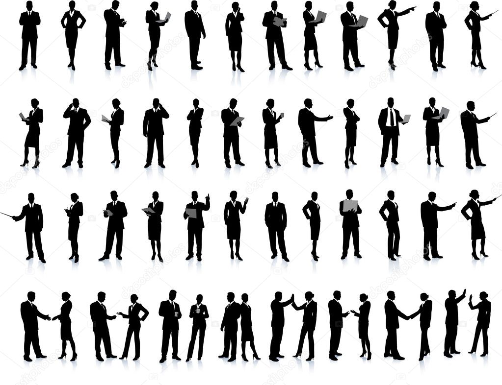
So I need human sized characters in my scene to give it some scale, there are various ways to do this, but I thought it'd be fun to write a little script that generates card people in various poses, heights etc. Doing a quick search on silhouette on Google Image search turns up this image at Deposit Photos, original link HERE,


Image 1: Various Silhouettes

I did a quick edit of the image to make it a square. Not too concerned with the watermarks.

Concept
1. Create shader using image 1 as opacity map
2. Create a polyplane with a dimension of 1x2 meters
3. Map the polyplane UV randomly to a person in image 1

Mel Script
global proc randCardPeople() {
    string $card1[];
    string $shaderName;
    string $shadingGroup;
    string $fileName;
    
    if (!(`objExists cardPeople`)) {
        $shadingGroup = `sets -renderable true -noSurfaceShader true -empty -name cardPeopleSG`;
        $shaderName = `shadingNode -asShader lambert -n cardPeople`;
        $fileName = `shadingNode -asTexture file`;

        connectAttr -f ($shaderName + ".outColor") ($shadingGroup + ".surfaceShader");
        connectAttr -f ($fileName + ".outColor") ($shaderName + ".incandescence");
        connectAttr -f ($fileName + ".outTransparency") ($shaderName + ".transparency");
    
        setAttr ($shaderName + ".color") -type double3 0 0 0 ;
        setAttr ($shaderName + ".diffuse") 0;    
        setAttr -type "string" ($fileName + ".fileTextureName") "/data/silhoutte.jpg";
        setAttr ($fileName + ".invert") 1;    
        setAttr ($fileName + ".alphaIsLuminance") 1;
    }


    $card1 = `polyCreateFacet  -p 0 0 0 -p 1 0 0 -p 1 0 -2 -p 0 0 -2 -name card`;
    rotate -r -os 90 0 0 ;
    makeIdentity -apply true -t 1 -r 1 -s 1 -n 0;

    sets -e -forceElement cardPeopleSG;
    select -r ($card1[0] + ".map[0:3]") ;
    polyEditUV -pu 0.25 -pv 0.5 -su 0.15 -sv 0.15;
    polyEditUV -u -0.25 -v -0.5; //move to 0 0
    polyEditUV -u 0.0613368 -v 0.355; //move to first row

    int $chooseU = `rand 12`;
    int $chooseV = `rand 1 4`;    
    polyEditUV -u (0.0815*$chooseU) -v (0.192*$chooseV);
    select -cl;
}

randCardPeople;

Conclusion


Results

Monday, October 8, 2012

MentalRay Custom Color Buffer / Linear Work Flow

Goal
Convert an existing mental ray shaded object into comp passes.

Introduction


Pic 1

In pic 1, we have the original shader.


Pic 2

In pic 2, we have the shader network. The top blinn is for the wooden base, the bottom material is for the porcelein/ceramic material. It consists of a fast_SSS connected to a mia_material, the color correction is to vary the front SSS color from the back SSS color.


Seperating the Passes
To reiterate, the goal is to recreate Pic 1 from passes.

Step 1: Create Passes
First lets go into Render Settings > Passes


Pic 3: Passes Window


Click on the first button on the right. It'll show a window with a list of different available passes. We'll just click on custom color, there are options to enter a prefix if needed. Rename the pass as "Diffuse". Do this another 3 times and name it as, "Refl", "SSS", "Spec". Once created, select all the passes and press the green check button in the middle of the Passes window. This will activate the passes.

Step 2: Rebuild the Shader Network
Lets do the wooden base shader first. This is simple blinn shader that consists of diffuse, specularity, and reflectivity.

Step 2A: Base Section
1. So let us create 3 writeToColorBuffer nodes in the hypershade. It can be found under the hypershade>create>mental ray>miscellaneous. Rename them as diffuse, spec, and refl. The custom color drop down list will contain a list of color passes we created in Step 1. Select the corresponding color passes for each writeToColorBuffer node.

2. Let us duplicate the blinn shader as well, since we can't output individual shading components from the blinn shader, we will need to re-create the shading components.


  • Diffuse: For the original blinn, turn reflectivity to 0 and specular color to black, and rename it diffuse.
  • Reflection: For reflection, create a mib_reflect under Sample Compositing
  • Specular: For the duplicated blinn, change diffuse to black and reflectivity to 0 and rename it to spec.


3. Now connect each of the blinn shader output to their corresponding writeToColorBuffer input. If you select all the nodes and graph it now, it'll show the pass nodes in the hypershade as well, as shown in pic 4.


Pic 4


4. If you render now, only the diffuse pass will show up since only the diffuse shader is connected to a shading group. One way for the other writeToBuffer node to evaluate is have the blinn somehow connect to the shadingGroup. But the official method is to use the evaluation passthrough of each writeToBuffer node.

  • Connect the refl node to the spec node, and the spec node to the diffuse node.
  • Disconnec the diffuse shader from the shading group
  • Create a surface shader and connect it to the shading group
  • Connect the diffuse writeToBuffer node to the surface shader input color.

It'll look something like in pic 5.


Pic 5


5. If we render now, it'll look like this,


Pic 6

The base will be black because of the surface shader. Here is what the passes look like,


Diffuse


Reflection


Specular


This concludes the base part.

Step 2B: Vase Section


  1. Create a SSS pass in render settings
  2. Create 4 writeToColorBuffer nodes and rename them as 2XSSS, refl, diffuse
  3. Upgrade the shaders,the vase part, I have a misss_fast_shader for diffuse and SSS, and a mia_material for the reflection. The misss shader is connected to the mia_material through additional colors. However, it would not matter once we use passes. These shaders are much easier to ouput passes since you can upgrade them to their respective X_passes shaders. The connections will be a little messed up but its easy to fix.
  4. Once upgraded, have the misss output front and back SSS results into to color buffers.
  5. Output diffuse result into the diffuse color buffer
  6. Output the reflection result from mia_material into the refl color buffer
  7. Disconnect materials from the shading group
  8. Create a surface shader and connect the last buffer node to the surface shader


pic 7
The final layout. 

Step 3: Render
Diffuse

Reflection

Specular

SSS
Combining the Passes
Once combined, you will notice that the combined passes will NOT look like the master beauty pass, this is due to the exposure mental ray adds to the beauty pass that is not added to the buffers. 

Comped Image

Master Beauty


To correct for this, we will need to upgrade our workflow to linear workflow.

Linear Workflow


  1. Change render settings > file format to exr
  2. Change render settings > quality > framebuffer to 4x16bit half in render settings
  3. Change render view > display > 32bit HDR
  4. Change render > display > color management, image color profile to linear, and display color profile to sRGB
  5. Color correct ALL texture/color swatch with a gamma correct node set to 0.4545


Comped Image

Master Beauty

The final shader network looks like this,


Final Shader Network

To have both master beauty and final passes rendered out, I connect the last outEvaluation to outMatteOpacity of the surface shader, doesn't effect anything but it will let it evaluate the passes. 

Notes I
There are limitations to custom color buffer workflow, some shading components from maya shaders will not output correctly and some might even interfere with other shading components. The safest way to ensure a consistent workflow would be to stick with mental ray shaders and keep it simple, after all, we're pretty much offloading the light tweak stage to the compositing department in this workflow.

Notes II
To improve the workflow it is advisable to standardize/limit the shaders used and also automate the pass and gamma correction process. Mel scripts will be provided.... when i get around to it.